Literature Review: Selection on soil microbiomes reveals reproducible impacts on plant function

I recently found an intriguing microbiome paper, and I would like to post my thoughts about it.

Citation
Panke-Buisse et al., Selection on soil microbiomes reveals reproducible impacts on plant function, ISME Journal 2014, doi: 10.1038/ismej.2014.196.

Review
The main hypothesis in this paper tests if phenotypes from a soil microbiome connected with a single plant genotype can be recapitulated in other plant genotypes.  First, early- and late-flowering time associated soil microbiome were generated.  Ten generations of Arabidopsis thaliana Col-0 were grown and at each generation soils from the four earliest and latests flowering pots were collected as the inoculum for the subsequent generation.  Using soils from generation 10, final early- and late-flowering time associated inoculums were derived.  These inoculums were then administered to four Arabidopsis thaliana ecotypes (Rld, Ler, Be, and Col-0) and a close relative, Brasica rapa.  Flowering time, plant biomass, and nitrogen mineralization enzyme activity for each of the genotypes were statistically different between early- and late-flowering associated inoculum treatments except Ler (Fig 4).  Microbes specifically associated with early- and late- flowering time treatments were found in low abundance suggesting that low-abundance microbes can contribute significantly to interesting phenotypes.


Positives In general, I found this paper to be very insightful for the following reasons:

• Soil Microbial phenotypes can persist in novel hosts.  This is a really cool result and could have direct implications for building field-useful microbiome treatments.  However, flowering time is a well conserved phenotype so this result may not apply to other specific phenotypes of interest such as crop yield, disease resistance, or with greater host genetic divergence (i.e. corn flowering time vs arabidopsis).
• Low abundance members of a community can drive an important phenotype.  A common assumption in metagenomics is that the most abundant members of a community are the most important.  Perhaps more focus should be geared toward linking microbes to phenotypes regardless of abundance.
• This artificial selection design doesn't require detailed knowledge of genetic mechanisms in order to produce a desired phenotype.  It is similar to the old dogma of plant breading where two good plants were crossed to produce an even better plant with no underlying knowledge of the genetic mechanisms.  While understanding the mechanisms is important for maximizing the phenotypic benefits, it is not required to generate a positive effect.

Critiques and Questions

• The methods section seems incomplete.
• Why are there so few OTUs in the heatmap and ternary plot?  Were OTUs filtered out?  I would expect to see hundreds or even thousands of OTUs from soil-derived microbiota.
• Were the wild soils combined at equal ratios?
• What was their measure of flowering time?  I think there are well defined methods in the literature for observing flowering time.
• Why are the EF associated samples in the 10 generation experiment actually flowering at a later time in later generations (supp fig 1)?
• Why are the control samples not included in supp fig 1?  
• Even though control samples were included as a covariate to generate figure 4, I would have liked to have seen them graphed there as well.
• Perhaps a better way of generating the control samples would have been to randomly pick pots to generate a control inoculum.  This was what they did in Swenson et al., 2000

Future Work
This experimental design could be used to address the following intriguing hypotheses:

• Selection on soil microbiomes changes the root endophyte microbial community.
• Redo the experiment with the same design but also 16S profile endophyte microbes.  
• It would also be interesting to see if the microbes specific to each treatment are also found inside the root.  This would suggest a direct microbial effect on the plant phenotype.
• Selection for soil microbiome associated phenotypes is driven by multiple mechanisms.
• Redo the experiment but don't combine replicates such that the end inocula include four independent lines of selection for both early- and late-flowering time soil microbiomes.  Compare microbes among treatment groups looking for different microbial profiles that express similar phenotypes.  

MiSeq Flow Cell Edges Correlate with Low Quality Scores

Upon receiving a FASTQ file fresh off the MiSeq, the first question I ask myself is:  "Did the sequencing work?"  On several occasions I open these files to discover the first few pages of sequence reads are littered with N's and have low quality scores.  However, when I run the full set of reads through a QC pipeline (e.g. FastQC) an overwhelming majority are high quality.

So why is it that the reads at the beginning of the FASTQ file have such poor quality?

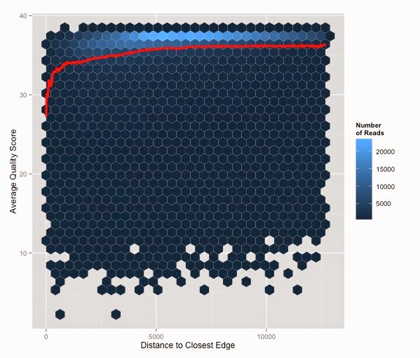
Reads generated using Illumina technology are ordered by their cluster's y-coordinate on the flow cell.  This led me to hypothesize that clusters near the edge of the flow cell are more likely to have low quality scores.  To test this hypothesis I took a subset of reads (932,709) from a MiSeq run, calculated their average quality score, and graphed that against the distance from the closest edge.

The splines function in R was used to model the relationship between average quality score and distance from the closest flow cell edge (red line).  Clusters closer to the edge of the flow cell have significantly lower quality scores.  However, the good news is that the vast majority of clusters do not fall close to the edge (light blue heat).  

In practical terms this issue is insignificant because so few reads are affected, but it does explain the high concentration of low quality reads at the beginning (and end) of Illumina generated FASTQ files.

When is my genome finished?

This is a common question for anyone doing genome sequencing and assembly.

The short answer:  never.

The slightly longer answer:  it depends.

The long answer:  Finishing a genome means the order of all nucleotide bases have been correctly resolved.  Even for simple genomes this is extremely difficult.  Billions of dollars have been spent to sequence the human genome, and it is currently estimated that 92% of the human genome has greater than 99.99% accuracy (Schmutz et al., 2004).  In total, 99% of the genome has been assembled, and the remaining 1% are likely to be highly repetitive regions with little or no gene content (remember that 1% of 3 billion total bases means there are about 30 million unresolved bases).  Using the current technology, it is impossible to reach 100% accuracy across 100% of the human genome.  For simpler genomes such as some viral and bacterial genomes it is possible to completely resolve the entire sequence.  However, because these genomes are much more dynamic (i.e. change at a faster rate), generating a completely finished genome may not be worth the cost.

Finishing a genome requires a substantial amount of time, work, and money.  However, getting a genome to draft status (i.e. incomplete but usable) can be done with minimal costs and resources.  So perhaps the most important question is:  when is my genome usable?  The answer to this question depends on the research questions being considered.  For example, when studying the evolutionary history of genomes with a high propensity for genomic rearrangements, generating long contigs/scaffolds is important for determining the orientation and lineage of genomic rearrangements.  Alternatively, some research questions are more concerned about the completeness of the gene content for making functional comparisons between genomes.  For such a question, generating long, continuous contig/scaffolds is less important.

Here are some possible ways to estimate completeness (with what I think are the best methods near the top):

• Compare the gene content of highly conserved genes
• Eukaryote:  CEGMA
• Bacterial:  CheckM
• Archaeal:  A table of 53 conserved COGs
• Check for possible errors using REAPR
• Calculate assembly metrics like contig number, N50, coverage, and assembly size.  
• Compare the size of your assembled genome to a related (or set of related) genome(s).  

See these papers for interesting discussion on evaluating assemblies:  

• Salzberg et al., 2011.
• Vezzi et al., 2012.
• Gurevich et al., 2013.
• Shangguan et al., 2013.
• Pan et al., 2014.

How to Order Contigs Using a Reference Genome

Background
In genomics complete (i.e. finished) genomes provide an excellent resource for future sequencing projects.  However, generating finished genomes is an expensive and laborious endeavor.  In some cases, the returns of finishing a genome are not worth the cost particularly when draft genomes can provide enough information for robust hypotheses testing.  Draft genomes contain a large number of unordered sequences of various lengths called contigs.  Contigs can be joined into more contiguous sequences called scaffolds using paired-end reads.  While a set of contigs/scaffolds can be useful for a wide variety of projects (gene annotation, gene expression profiling, etc.), contig order provides vital information in comparative genomics and analyses of specific genomic regions.  Typically, a rough ordering of contigs can be accomplished by mapping contigs to a closely related reference genome.

ABACAS
Recently, I discovered a nice software package called ABACAS which not only orders contigs but creates a contiguous sequence representing the connected contigs.  Gaps between contigs are represented by N's and overlapping regions are resolved (although I could not find information on exactly how).  Because ABACAS requires MUMer, its outputs integrate will with other MUMer scripts such as those for visualizing alignments (Figure 1, i.e. mummerplot).  ABACAS is hosted by SourceForge and is well documented.  It was published in Bioinformatics in 2009.

Notes
Of course, more closely related draft and reference genomes will generate the most correct ordering.  However, in cases where the target genome is VERY closely related to the reference genome it may be better to map raw reads to the reference genome instead of build a de novo assembly.  Deviations from the reference genome can be discovered using SNP detection software.  Read mapping experiments are generally cheaper because they require fewer reads than de novo assembly but can still detect biologically significant differences when compared to the reference genome.

Cool Unix Commands

I will add to this list as I discover new ones.  If you have a favorite or useful command feel free to include it in a comment on this post.

Convert a FASTQ file to FASTA (originally posted here):

sed -n '1~4s/^@/>/p;2~4p' 

NOTE: this assumes that each FASTQ entry spans only four lines as is customary.



Convert a SAM file to FASTA

awk '{OFS=""}{print $1, "\n", $10; }' file.sam > file.fasta

NOTE: You will loose a lot of information in the sam file.  You can save more of that info by adding column variables to the print statement.  Also, you may have to change the column variable numbers depending on your sam file format.  This is just a general example.



Replace spaces in file names with underscore (originally posted here)

rename ' ' '_' *

NOTE:  do NOT put spaces in file names!!  This is so annoying!



Get a histogram of sequence lengths from FASTA/Q files (from Surge Biswas)

FASTQ:  cat <fastq file> | awk '{if(NR%4==2) print length($1)}' | sort -n | uniq -c
FASTA:  cat <fasta file> | awk '{if(NR%4==0) print length($1)}' | sort -n | uniq -c



Do arithmetic operations on the bash command line

echo $((1 + 1))
echo $((1 - 1))
echo $((1 * 1))
echo $((1 / 1))
echo $(((1+3) / (1+1)))

For floating point operations you can use the bc tool.  For example

echo "scale=1; 1/2" | bc



Add a comment to a bash command on the command line

<command>; # this is a comment line

A practical example:  mv file1 old_file1; # there is now a new file1 is a more recent version

NOTE:  Do you ever have a long and complex command for which you would like to save a simple note?  You can use this little trick and the note will be saved along side your command in your history.  The next time you look through your history to rerun the command you will also see the associated note.



Count the number of bases in a FASTA file

grep -v ">" file.fasta | wc | awk '{print $3 - $1}'

(from martinghunt on SEQanswers)

How to Learn Bioinformatics

Introduction

At least once a month someone asks me for help learning bioinformatics.  I love it when this happens because it usually means they want to take control of their own analysis thereby freeing up my time for problems that interest me.  This post is a collection of tips and resources for people wanting to learn how to do bioinformatics.

Keep These Things in Mind:

• Learning the basics of bioinformatics is easy.  The basics as described in this post are often taught in high school.  However, don't get frustrated if you don't understand everything all at once.  Learning anything new takes time and practice no matter its difficulty.  
•  A little bit goes a long way.  I estimate that nearly 90% of my work is occupied by simple routine procedures.  Learning how to do these tasks will substantially expand your ability to analyze and interpret your data.
• Google it.  Google is the best resource for learning new techniques and trouble shooting problems.  If you have a question type exactly what you would say to a person into the google search bar.  When you take questions to your bioinformatics friends it's likely they won't know the answer offhand and will google it anyway.
• Try it.  If you're not sure about something try it and see what happens.  Generally, there is very little danger is just trying a command to see if and how it works.  That being said it's a good idea to backup important files and data just incase something goes very wrong.  Every Unix programmer that I know has deleted a really important file using the rm command (which is one of the few irreversible Unix commands).  It's going to happen to you too so make a backup.

Learn the Unix Basics

• Get on a Unix machine.  Doing is the most important aspect of learning Unix.  You will never fully understand the basic concepts if you only read about them.  Mac users have it easy because OSX is build on a unix shell.  Simply open the terminal application and you are ready to start with an online tutorial.  For non-mac users I recommend finding an old computer and installing a Linux/Unix operating system like Ubuntu.  A slightly more difficult approach would be to partition the drive of an existing computer to dual boot a Linux/Unix OS along with the existing OS.
• Complete an online tutorial
• Unix Tutorial for Beginners
• Introduction to Unix for Biologists
• Unix and Perl Primer for Biologists

• Buy a book if you are a book learner.  However, the basic can pretty much all be learned using online materials.  My favorite Unix book is O'Reilly's Unix Power Tools.

Learn a Scripting Language

• Pick a scripting language.  Scripting languages are computer languages that are not compiled (i.e. they are interpreted by the computer on the fly).  The two most popular bioinformatics scripting languages are Perl and Python.  Both languages have their strengths and weakness, but I personally prefer Perl.
• Complete an online tutorial for your language.
• Perl tutorial
• Perl and Unix for Biologists
• Python tutorial
• Python for Biologists
• Buy a book.  My favorite Perl book is Perl Best Practices by Damian Conway.  This book is a must have for all Perl programmers!  I don't have much experience with Python books, so I would recommend looking at book reviews before making a purchase.

Learn a Statistical/Graphing Language

• Pick a language for doing statistical operations and building figures.  Languages like R and Matlab are prime choices for both statistics and graphics.  Both languages have their strengths and weaknesses, but I personally prefer R.  If you choose R I highly recommend using the ggplot2 library for building figures.  
• Complete an online tutorial for your language.
• R tutorial (ggplot tutorial) (another fantastic R tutorial by DataCamp)
• Matlab tutorial 
• Give up Excel.  Excel is a powerful program but lacks the flexibility of computer languages like R and Matlab.  While there is a steeper learning curve for R and Matlab, you will substantially enhance your ability to do statistical analyses and build graphics by getting away from Excel.

Learn Basic Bioinformatics Procedures and Corresponding Software Tools

For example:

• Quality control
• fastQC
• Sequence assembly
• Velvet,
• SPAdes (my preference, also see this post)
• Sequence mapping
• BWA
• Bowtie
• Sequence searching
• BLAST
• Differential expression
• edgeR
• DESeq
• Variant calling
• GATK
• etc

This is only a small list of procedures and tools primarily focusing on DNA sequence analysis.  For a more comprehensive list see OMICtools.


Find a problem

I strongly encourage new bioinformaticians to find some real data to do meaningful science using the above principles and skills.  If you don't personally have data I recommend downloading data from a public repository (i.e. Genbank).  A similar alternative would be to choose a paper that uses a procedure you are interested in learning and recapitulate the results.  

Predicting Full-Length Ribosomal Gene Sequences

Introduction

The 16S ribosomal gene has been used extensively in biology for distinguishing relatedness between species.  This gene has regions of DNA that are highly conserved among almost all living organisms and other regions that have high DNA sequence variability.  The conserved regions are ideal for building PCR primers that can amplify DNA from many different organism.  The variable regions that are amplified using these conserved primers can be used to determine the relatedness between two or more organisms.  Closely related species typically have much more similar DNA sequences than distantly related species.

Typically PCR is used to amplify a portion of the 16S ribosomal gene for sequencing.  However, whole genome sequences or whole metagenome sequences also contain short DNA reads originating from the 16S gene.  These reads can be separated from the pool of other genomic reads and assembled into the entire 16S gene.  EMIRGE (Miller, et al. 2011) is an algorithm for reconstructing full-length ribosomal genes from short read DNA sequences.


EMIRGE

EMIRGE reconstructs full-length ribosomal genes from short read DNA sequences.  It first maps reads to a database of known 16S genes such as the SILVA or greengenes database.  After the initial mapping, EMIRGE estimates the probability that a given read was generated from the reference to which it mapped.  Based on these probability estimates, reference sequences are changed to reflect the 16S sequences that are likely to be represented by the set of reads.  Reads are then remapped to the adjusted 16S sequence database and the processes is repeated until an equilibrium is achieved.  The resulting database of 16S sequences reflect the likely 16S genes represented by the input set of short reads.

This software was primarily built to infer the set of 16S genes from whole metagenome reads.  However, it can also be used to infer the single 16S gene from genomic sequences from a single isolate.  Full-length 16S genes are difficult to assemble even when only reads from a single genome are considered.

In the Dangl lab, we use EMIRGE to predict full-length 16S genes from reads generated from a single genome of bacteria.  An example of the EMIRGE command we use is:

emirge.py my_output_dir -1 fwd_reads.fastq -2 rev_reads.fastq -b SSURef_NR99_115_tax_silva_formated -f SSURef_NR99_115_tax_silva_formated.fasta -i 600 -s 1000 -l 250

The descriptions of each parameter are below:

my_output_dir: the output and working directory for EMIRGE.

-1: the forward or single-end genomic sequencing reads

-2: the reverse end genomic sequencing reads

-b: the bowtie index of the 16S sequence database

-f: the fasta file of the 16S sequence database

-i: insert size of paired-end reads

-s: standard deviation of insert size for paired-end reads

-l: max length of reads


Other Details

EMIRGE uses bowtie to map reads to the reference database.  To build the bowtie index of the reference database the following command was used:

bowtie-build SSURef_NR99_115_tax_silva_formated.fasta SSURef_NR99_115_tax_silva_formated

Also, the database downloaded from SILVA had to be reformatted using this Perl script.  This script requires BioUtils.